BlueCap Australia

BlueCapLidar® Drone LiDAR System

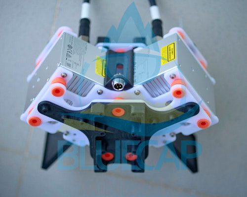
BlueCapLidar® is a high-productivity Drone LiDAR system for terrain mapping and surface model generation in steep exploration terrain.

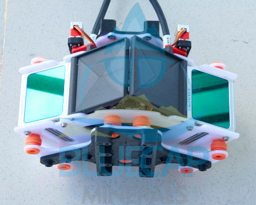
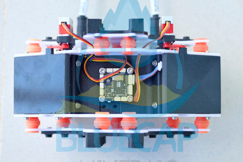
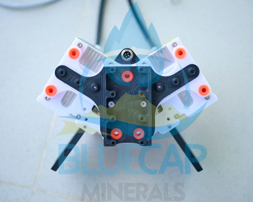
BlueCapLidar® dual-sensor payload for terrain mapping

Drone LiDAR equipment for high-productivity terrain mapping

BlueCapLidar® is an in-house system built around four connected elements:

  • Payload: two DJI Livox® Avia LiDAR sensors in one swappable basket.
  • Carrier: the BlueCapHeli® drone helicopter, with the basket isolated on vibration dampers.
  • Recording: an onboard microcomputer and 2 TB SSD capture point clouds, IMU parameters and RTK positioning data together.
  • Survey role: rapid mapping of terrain, canopy and obstacles for large-area LiDAR and safer low-level magnetic acquisition.
285 × 160m · 45,600 m² (4.56 ha)
Instantaneous surface footprint at 100 m AGL
90–540km²/day
9,000–54,000 ha/day
250pts/m²
Dual-orthogonal grid density · two perpendicular line sets
BlueCapLidar® dual-sensor payload

BlueCapLidar®

Real-world LiDAR system comparison

BlueCap has run controlled system comparisons in the field. The first matrix isolates the principal hardware figures; the commercial field-time comparison follows immediately below it.

Field comparison basis: 100 m AGL · one-direction parallel lines · eight-hour field day · line turns and return-to-base included · complete refuelling or battery-service cycles.

Real-world LiDAR system comparison for geophysicists and large-area mapping teams
Comparison criterionBlueCapLidar®ROCK R3 V2DJI Zenmuse L2
Scanner2 × Livox AviaHesai XT16 · 16 channelsIntegrated frame LiDAR
Point output · million points/s1.440.641.20
Inertial architecture · IMUs411
Surface window at 100 m AGL285 × 160 m · 45,600 m² · 4.56 ha120 × 35 m · 4,200 m² · 0.42 ha140 × 153 m · 21,420 m² · 2.14 ha
GNSS Accuracy · RTK0.8 cm1 cm1 cm
ApplicationsUrban · mining · exploration · corridors · LiDAR + magneticsAerial · vehicle · handheldTopography · forestry · power lines
Field economics · eight-hour field day

How LiDAR productivity changes field days and project cost exposure

Figures are not guaranteed production rates. They are experience-based planning values grounded in BlueCap controlled field comparisons and the recorded operating histories of experienced LiDAR crews.

Experience-based BlueCapLidar® and DJI Zenmuse L2 field-time comparison
Survey blockBlueCapLidar®carried by BlueCapHeli®Zenmuse L2carried by DJI Matrice 300 RTK
10 × 10 km100 km²
8.9 hflight time
2field days
4flight legs
3refuels
77 hflight time
13field days
165battery flights
20 × 20 km400 km²
35.6 hflight time
5field days
15flight legs
14refuels
307.5 hflight time
51field days
659battery flights
30 × 30 km900 km²
80 hflight time
10field days
32flight legs
31refuels
692.1 hflight time
115field days
1483battery flights

BlueCapHeli® basis: The conservative case uses 90 km² in an eight-hour field day. Each fuelled flight leg lasts 2.5 hours and covers 28.125 km² in this planning case.

DJI operator basis: The calculation uses an operator-reported 150 acres (60.7 ha) in a 28-minute mission at 100 m AGL, 10 m/s and 50% sidelap with Zenmuse L2 on the Matrice 300/350 class. A second L2 operator reports 80–100 ha per battery at 100 m AGL and 15 m/s. The lower observed result is used, including mission turns and return-to-base; an eight-hour field day allows 13 complete battery-flight and service cycles. 60.7 ha field report ↗ 80–100 ha cross-check ↗

Operator cross-checks: Matrice 300/350 with Zenmuse L2 and ROCK R3 Pro V2 field experience; L2 mission at 100 m AGL, 10 m/s and 50% sidelap.

What it is

Vibration-damped dual-sensor suspension for two DJI Livox® Avia-class sensors.

Purpose-built medium-sized LiDAR platform for long-endurance operation in remote exploration terrain.

Down-looking, nadir-focused laser scanner geometry designed to maximize useful ground returns for bare-earth DEMs in vegetated and steep terrain.

Protected optics for field deployment: LiDAR optical windows remain covered during take-off and open only after climb-out, reducing dust contamination.

4-IMU fusion: exactly four IMUs — one in each of the two DJI Livox® Avia sensors, one on the BlueCapLidar® basket and one on the carrier platform — are fused with RTK GNSS positioning of 0.8 cm horizontally.

Edge to cloud processing workflow: LiDAR batches, telemetry and QA data are staged for CPU-cluster processing and project deliverables.

The complete system is carried by a medium-sized helicopter-class BlueCapHeli® drone helicopter with the LiDAR basket isolated on vibration dampers.

Status: The Drone LiDAR equipment is operational and being field-validated through selected pilot projects. The priority is measured performance, repeatable workflow and defensible survey outputs rather than demonstration-only flights.

Where BlueCapLidar® fits

BlueCapLidar® is a large-area mapping system, not only a magnetic pre-survey payload. Its wide instantaneous surface view and BlueCapHeli® endurance support two connected applications:

  • Conventional large-area LiDAR: urban districts · mining areas · exploration blocks · transport and utility corridors · remote infrastructure · broad terrain-model programs.
  • Integrated geophysics: the same terrain products feed directly into low-level BlueCap magnetic survey planning.

Why LiDAR comes before a magnetic survey

BlueCapLidar® first creates a high-accuracy terrain and obstacle model.

Absolute accuracy (single-pass)

  • XY: 3–5 cm
  • Z: 4–8 cm
  • Z under canopy: ≤10–15 cm

Absolute accuracy (dual-orthogonal)

  • XY: 1.5–2.5 cm
  • Z: 2–4 cm
  • Z under canopy: ≤7 cm

The BlueCapHeli® drone helicopter, its active BlueCapWinch® and the pre-planned flight trajectory then work as one control system. Together they carry the BlueCapBird® magnetometer along the calculated drape surface and deliver ±1 m terrain-following accuracy relative to the LiDAR model.

For drone magnetic surveying, this is a data-quality requirement: the LiDAR surface model defines the profile used for drape planning, speed control and sensor-AGL quality control before low-level magnetic acquisition.

  1. Map the surface at 100 m AGL

    BlueCapLidar® records a 285 × 160 m instantaneous surface window and builds the terrain and obstacle model before the magnetic flight.

  2. Calculate the magnetic drape

    The model converts terrain, canopy and obstacles into a flyable sensor-height profile. A 35 m sensor AGL reference represents a common operating clearance in difficult mountainous and hilly tropical or subtropical terrain.

  3. Control the suspended sensor

    BlueCapWinch® actively manages the Quantum Rubidium Atomic Magnetometer, QuSpin QTFM Gen 2, while maintaining more than 20 m carrier-to-sensor separation.

  4. Fly and verify to ±1 m

    Acquisition follows the calculated drape, with speed control and AGL quality checks used to limit terrain-following error before geophysical interpretation.

Field experiment: terrain-following error can masquerade as geology

BlueCap repeated a controlled experiment at four separate field locations. At each location, the BlueCapHeli® drone helicopter hovered above one fixed horizontal point while BlueCapWinch®, its active winch, raised and lowered a Quantum Rubidium Atomic Magnetometer, QuSpin QTFM Gen 2, through 25–50 m sensor AGL. BlueCapWinch® actively controlled the suspended sensor height. Throughout the experiment, the sensor never approached the BlueCapHeli® airframe closer than 20 m. Every height below is the magnetic sensor height above ground, not the carrier altitude.

  • Four field locations

    The controlled vertical profile was repeated at four separate locations rather than inferred from one site.

  • Fixed horizontal position

    The carrier remained above one point while only the sensor–ground separation changed.

  • BlueCapWinch® height control

    The active BlueCapWinch® controlled the suspended Quantum Rubidium Atomic Magnetometer, QuSpin QTFM Gen 2.

  • Controlled separation

    Sensor AGL cycled from 25 to 50 m, while carrier-to-sensor separation remained greater than 20 m.

Geophysical interpretation of the height response

For a compact shallow source observed at distances large relative to the source dimensions, the magnetic field may be treated to first order as a dipole field. Along a comparable observation geometry, anomaly amplitude decays approximately as r⁻³, where r is sensor–source separation. Consequently, vertical positioning error is multiplicative rather than additive: reducing sensor AGL increases short-wavelength anomaly amplitude, while increasing sensor AGL attenuates it and shifts the effective spectral response.

The chart normalises the 35 m sensor-AGL response to 100% and evaluates the first-order r⁻³ relationship across the 25–50 m AGL range used in the BlueCap experiment. The 35 m reference is a common sensor operating height in difficult mountainous and hilly terrain in tropical and subtropical environments. This is a geophysical interpretation of the controlled experiment, not a substitute for the unpublished raw time series from the four locations. The result demonstrates how terrain-following error can introduce amplitude variation that may be misinterpreted as geology.

BlueCap field experiment · normalized interpretation

Normalized height-response curve

The curve sets the 35 m sensor-AGL response to 100% and applies the first-order 1/r³ relationship across the field-tested 25–50 m range. It interprets the controlled experiment; it is not a plot of the unpublished raw series from the four locations.

25 m30 m35 m40 m45 m50 m0%50%100%150%200%250%300%~274%~159%100%~67%~47%~34%Normalized anomaly response (% of 35 m sensor-height reference)QuSpin sensor height above ground (m AGL)
Normalized 1/r³ reference across the field-tested height range ±1 m terrain-following control band using a BlueCapLidar® surface model Reference at 35 m sensor AGL = 100%

The operational conclusion is direct: pre-survey LiDAR constrains the terrain surface before acquisition, allowing amplitude changes caused by sensor-height error to be distinguished from the geological response. Competing systems may produce a valid point cloud; BlueCap's differentiator is the closed workflow from surface measurement to magnetic drape planning, acquisition and AGL quality control.

45,600 m² (4.56 ha) instantaneous LiDAR footprint at 100 m AGL

At each instant, the dual-sensor BlueCapLidar® geometry projects a surface-view window approximately 285 m wide × 160 m along track at 100 m AGL over SRTM-referenced terrain.

This is the surface visible to the LiDAR at one moment, not an area-per-second value or a completed survey production rate.

  • Flight speed
  • Line overlap
  • Terrain and canopy
  • Required point density
285 m across track
160 m along track
45,600 m²4.56 havisible at one moment
Instantaneous projected surface window · 100 m AGL
Official product photograph of the ROCK R3 drone LiDAR package
ROCK R3 V2
Same altitude · speed · flight time

Direct ROCK R3 V2 comparison

BlueCapLidar® uses two DJI Livox® Avia sensors set 32° apart. The comparison holds the flight basis constant and separates instantaneous geometry, point output and time-based production.

  • BlueCapLidar® instantaneous view285 × 160 m = 45,600 m² at each moment at 100 m AGL.
  • ROCK R3 reference view120 × 35 m = 4,200 m² under the same BlueCap geometric assumption at 100 m AGL.
  • Registered point outputBlueCapLidar® records 1.44 million reflected points/s; ROCK R3 V2 records 0.64 million points/s. BlueCapLidar® therefore records 2.25 times the reflected-point rate.
  • Production interpretationAt 100 m AGL, BlueCapLidar® sees 45,600 m² at one moment versus the 4,200 m² ROCK reference. The 10.9 times ratio compares only the instantaneous viewing windows; completed hourly coverage also depends on speed, overlap, turns and required density.

The useful comparison is not the nominal 360° rotating scan envelope. It is the ground-observation geometry and usable return density achieved beneath the aircraft for the same mission basis.

Dense canopy: four viewing directions, not two

In dense tropical vegetation, one pass from one direction may not place enough laser pulses through gaps in the canopy. BlueCap therefore flies a second pass at 90° to the first. The dual-orthogonal pattern observes objects from four directions rather than two, increases ground returns and improves DSM detail.

Two perpendicular line setsFour viewing directions sample different openings instead of repeating the same two-sided view.

At 100 m AGL and 80 km/h, 250 pts/m² is the dual-orthogonal grid density: the area is flown with two perpendicular sets of parallel lines, like graph paper. It is not the density claim for an ordinary one-direction set of parallel flight lines. BlueCapLidar® can complete this dual-orthogonal pattern in the time a ROCK R3-class system requires for a conventional single-pattern survey, delivering twice the directional acquisition within the same operational window.

In-house processing avoids proprietary integration hours

BlueCapLidar® and its post-processing workflow are developed by the same BlueCap team. The system records standard point-cloud and flight data into the in-house MCAP/MavROS 2 workflow, so client-specific changes can be made directly by the engineers responsible for the payload.

For comparison, integrating third-party proprietary hardware and software can consume dozens or hundreds of engineering hours in vendor training, data adaptation and custom changes. At BlueCap's client post-processing rate of AUD 290 per hour, avoiding that integration burden is a material project-cost issue, not only a software preference.

Drone LiDAR system performance envelope

Parameter
BlueCapLidar® value
Practical meaning
ParameterNominal operating altitudeBlueCapLidar® value100 m AGL over SRTM-referenced terrainPractical meaningHigh-productivity terrain mapping height used for the footprint and coverage figures below.
ParameterInstantaneous projected surface footprintBlueCapLidar® valueApprox. 285 m wide × 160 m along track at 100 m AGL over SRTM-referenced terrainPractical meaningThe surface window visible to the dual-sensor geometry at each moment.
ParameterInstantaneous projected footprint areaBlueCapLidar® valueApprox. 45,600 m² (4.56 ha) at 100 m AGLPractical meaningGeometric area of the 285 m × 160 m surface window; not an area-per-second rate.
ParameterTypical survey speedBlueCapLidar® value80-100 km/hPractical meaningProduction speed range; platform limit is approximately 140 km/h.
ParameterPoint densityBlueCapLidar® valueApprox. 100-120 pts/m² in a single production pass; approx. 250 pts/m² with orthogonal dual-pass at 100 m AGL over SRTM-referenced terrain and 80 km/hPractical meaningSupports DEM/DSM extraction and dense-vegetation workflows.
ParameterSensor layoutBlueCapLidar® valueDual DJI Livox® Avia LiDARs mounted with a 32-degree angle between sensors, using angled nadir-focused geometryPractical meaningDesigned to maximize useful ground returns rather than full-sphere scanning.
ParameterPoint outputBlueCapLidar® value1.44 million reflected points per secondPractical meaningSecondary sensor metric; useful when considered together with ground footprint and mission geometry.
ParameterPositioningBlueCapLidar® valueRTK GNSS with 0.8 cm horizontal accuracy; 4-IMU fusion: exactly four IMUs — one in each DJI Livox® Avia, one on the BlueCapLidar® basket, and one on the carrier platformPractical meaningSupports precise sensor position and attitude for point-cloud processing and terrain-aware magnetic survey planning.
ParameterProcessingBlueCapLidar® valueAutomated tiling with 20 m overlaps; overnight CPU-cluster processing, approx. 4 h typical for a day of LiDAR dataPractical meaningDesigned for practical project delivery rather than isolated demonstration flights.
ParameterAssumptionsBlueCapLidar® value100 m AGL over SRTM-referenced terrain, terrain-mapping production mode, dual-sensor nadir-focused geometryPractical meaningFigures describe useful ground observation, not total theoretical scanner FOV.

Deliverables

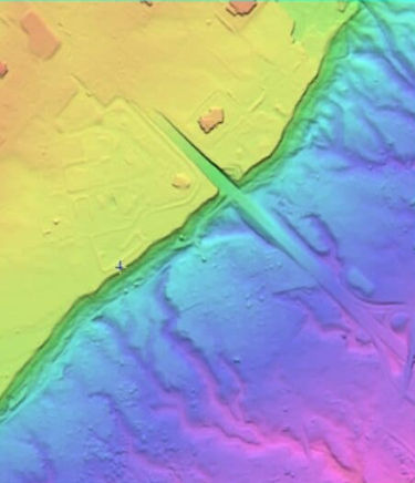
Bare-Earth DEM (vegetation removed) – GeoTIFF

Canopy/Surface DSM – GeoTIFF

Obstacle Vector Map – powerlines, poles, towers, buildings, tree crowns (format by request)

Intensity Tiles & QA layers – by request

Coordinate & vertical datums: project-specific (EPSG/ellipsoid/geoid agreed in advance)

File formats: LAS/LAZ 1.4, GeoTIFF; standard tile sizes (e.g., 1 × 1 km)

Workflow

  1. Reconnaissance LiDAR flights

    Reconnaissance LiDAR flight(s) → raw point clouds

  2. Automated processing

    Automated processing on a multi‑node CPU cluster

  3. Terrain and obstacle models

    DEM/DSM & obstacle maps generated and validated

  4. Mission planning

    Mission planning: terrain‑aware line design with speed/altitude envelopes

  5. Magnetics deployment

    Magnetics deployment: long‑endurance flight missions at higher throughput

LiDAR Integration with magnetic surveys

DEM-assisted draping: terrain-aware flight lines help maintain consistent magnetic sensor clearance over steep ground.

Quality control for geophysicists: LiDAR-derived terrain lets the interpretation team separate geology-driven magnetic amplitude changes from flight-geometry artefacts.

Higher field productivity: known terrain and obstacle envelopes reduce start/stop events, pilot workload and conservative slow-flight segments.

Bundled workflow: the same team can plan terrain mapping, magnetic acquisition and deliverable requirements, reducing handover errors between contractors.

Field validation data

For geophysicists and project managers, the most persuasive evidence is measured data. BlueCapLidar® should be evaluated by the same deliverables it produces for magnetic survey planning.

Validation item
What it proves
Status / next step
Validation itemPoint cloud screenshot and cross-sectionWhat it provesCanopy penetration, ground returns and surface structureStatus / next stepAvailable from pilot datasets / supplied on request
Validation itemBare-earth DEM and canopy DSM sampleWhat it provesTerrain model quality for drape planning and magnetic correctionsStatus / next stepPrepared per project area and datum
Validation itemObstacle vector exampleWhat it provesDetection of powerlines, towers, buildings, tall trees and other flight hazardsStatus / next stepFormat by request for mission planning workflows
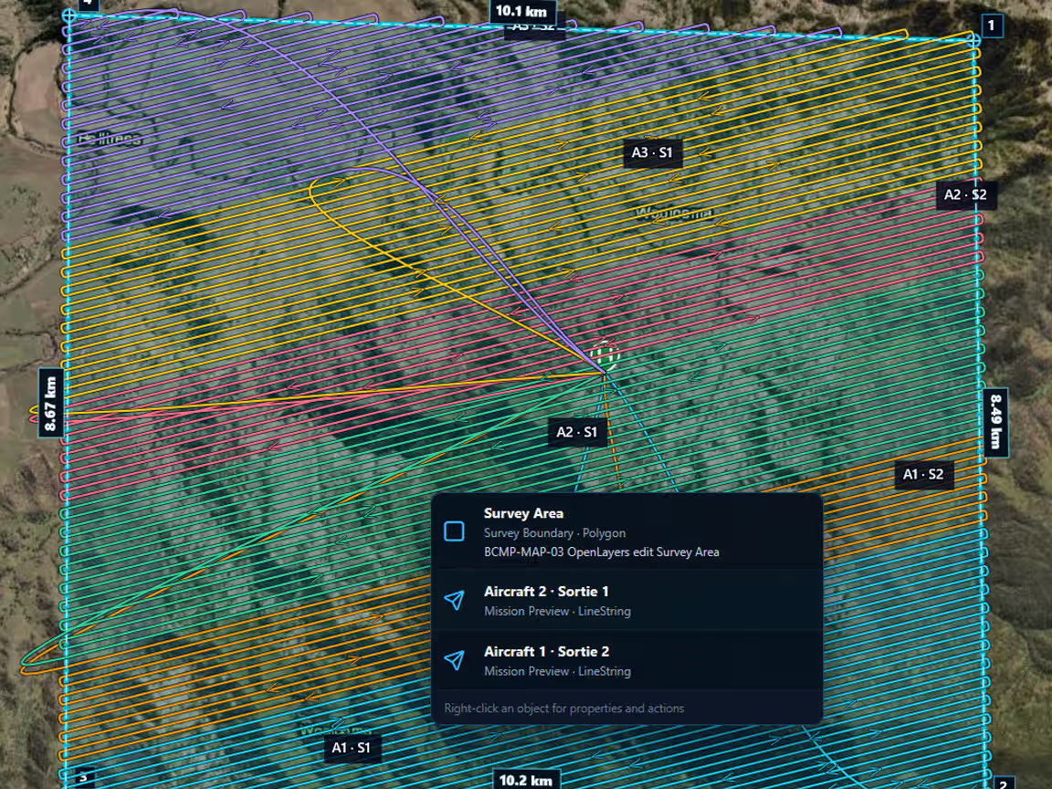
Validation itemFlight path plus footprint overlayWhat it provesActual flight path, instantaneous footprint and accumulated coverage geometryStatus / next stepUsed internally for mission planning and client review
Validation itemSample LAS/LAZ or GeoTIFF tileWhat it provesIndependent technical review by client geophysicists or GIS teamsStatus / next stepAvailable for selected projects under data agreement

Commercial impact for exploration projects

BlueCapLidar® is designed to improve the economics of exploration surveys, not only the appearance of terrain data. In remote projects, the expensive constraint is often the number of flyable hours, field crew days and repeat visits caused by uncertain terrain or unreliable magnetic data.

Commercial risk
How pre-survey LiDAR helps
Investor / client relevance
Commercial riskShort weather and airspace windowsHow pre-survey LiDAR helpsFlight-plan modelling combines footprint, speed, overlap, terrain and required density.Investor / client relevanceMore productive field days and lower standby cost.
Commercial riskIncorrect magnetic target positioningHow pre-survey LiDAR helpsBetter drape planning reduces AGL-driven anomaly distortion.Investor / client relevanceLower risk of drilling decisions based on flight-geometry artefacts.
Commercial riskRepeat surveysHow pre-survey LiDAR helpsIntegrated LiDAR plus magnetic workflow improves planning before acquisition.Investor / client relevanceFewer re-flights and cleaner handover to interpretation teams.
Commercial riskContractor handover gapsHow pre-survey LiDAR helpsThe same team understands LiDAR terrain products and magnetic survey requirements.Investor / client relevanceStronger defensibility for professional exploration programs.

Availability & pricing

Availability: limited pilot projects during field‑testing; priority to sites that help validate edge cases (dense canopy, steep relief, high line density).

Pricing: scoped per site area, relief, vegetation, and deliverables; indicative budgets on request. Bundled LiDAR + Magnetics pricing available.

Technical notes

Nadir-oriented scanning is preferred for reliable ground returns in vegetation; forward-looking LiDAR tends to bias returns toward canopy projections and visible slopes.

Bare-earth extraction relies on sufficient multi-angle coverage and ground-level return density; overlap, speed and flight geometry are tuned per terrain and vegetation type.

The 285 m × 160 m figure is the instantaneous projected surface window at 100 m AGL. It is not an area-per-second rate; production estimates also require speed, overlap, terrain, scan pattern and required density.

Processing priority: quality-controlled deliverables are processed on CPU workstations or clusters; real-time onboard classification is not required for the survey objective.

Project enquiry

Start with the survey decision

Share the target area, terrain, line spacing, required outputs and operating constraints. We will review whether the project is a suitable fit.

  1. Define the survey

    Survey boundary, access points, terrain context and operating constraints.

  2. Build the scope

    Coverage geometry, line distance, duration and project inputs.

  3. Design the mission

    Terrain-aware flight lines, altitude, speed and sensor geometry.

  4. Acquire and review

    Field acquisition progress, preliminary coverage and QA/QC indicators.

  5. Process and deliver

    Processing outputs, approved reports and final datasets.