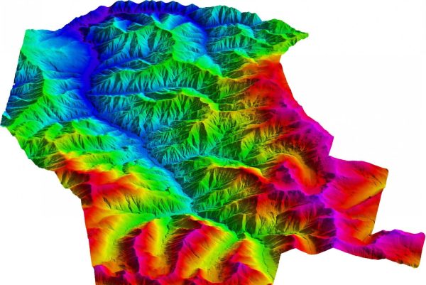
01 Drape terrain · ≈150 pts/m²
Single pass · 120 m AGL · 100 km/h · fast DEM for the magnetic drape
- Line-km / week
- ≈10,200
- km² / day
- ≈305
- km² / week
- ≈1,530
BlueCap Australia
LiDAR mapping built for mineral exploration and mining, mine planning, telecommunications and infrastructure — from broad terrain programmes to detailed corridor and site mapping.
SENSOR-CENTRIC FULL-PHYSICS PLANNING
Our sensor-centric physical simulation calculates the terrain-following trajectory and acquisition geometry before take-off, combining exceptional precision with the area coverage of the BlueCapHeli® system.
Explore survey planningLiDAR survey · LiDAR mapping · terrain models · point clouds · QA
BlueCap provides drone LiDAR survey and mapping services for mineral exploration, mining and infrastructure across Australia and worldwide. The BlueCapLidar® drone LiDAR system and long-endurance aircraft connect acquisition to classified point clouds, bare-earth terrain models and reviewable QA. LiDAR is one of the three methods in BlueCap's drone survey and mapping services across Australia, flown from the same aircraft as aeromagnetic and radiometric acquisition.
Four planning numbers connect field capacity, parallel deployment, point density and processing turnaround.
12,000–30,500 ha across an eight-hour field day with one BlueCapHeli® survey system, from cross-grid detail to drape terrain.
One BlueCapHeli® survey system plans three helicopters as a coordinated field team; the project plan determines how they operate.
The project range runs from drape terrain at 120 m AGL to a dual-orthogonal canopy survey at 100 m AGL and 80 km/h.
Field acquisition is visible in the browser; controlled terrain processing continues after each flight.
Three acquisition tiers, one system. Drape terrain is the fast tier that turns a block into a DEM for the magnetic drape within days of mobilisation; the detailed tiers fly lower and slower, once or twice at 90°, for canopy, outcrop and engineering-grade surfaces. Figures are planning values for the BlueCapHeli® system over five flying days.
Single pass · 120 m AGL · 100 km/h · fast DEM for the magnetic drape
Single pass · 100 m AGL · 80 km/h · terrain, canopy height, infrastructure
Two passes at 90° · 100 m AGL · 80 km/h · dense canopy, outcrop, engineering surfaces
| Acquisition tier | Line-km / week | km² / day | km² / week |
|---|---|---|---|
| 01 Drape terrain · ≈150 pts/m²Single pass · 120 m AGL · 100 km/h · fast DEM for the magnetic drape | ≈10,200 | ≈305 | ≈1,530 |
| 02 Detailed · ≈230 pts/m²Single pass · 100 m AGL · 80 km/h · terrain, canopy height, infrastructure | ≈8,150 | ≈245 | ≈1,225 |
| 03 Detailed cross-grid · ≈455 pts/m²Two passes at 90° · 100 m AGL · 80 km/h · dense canopy, outcrop, engineering surfaces | ≈8,150 | ≈120 | ≈610 |
Densities are nominal per-pass values in the single-coverage part of the swath, before sidelap gain, canopy losses and ground classification; about 6.8 productive hours per 8-hour flying day are assumed. Terrain, canopy, airspace, weather and turns are confirmed in the quotation.
Define the survey area, plan routes, develop a quote-ready scope, follow field acquisition and keep processed results and deliverables in one connected project workspace.
Dual-sensor point clouds, four-IMU data, RTK positioning and flight telemetry remain connected in the same synchronised field record.
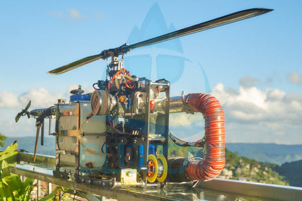
The hybrid petrol-powered carrier provides 3 or 8 hours of endurance, field refuelling and a normal 100 km/h cruise speed for productive survey acquisition.
The BlueCap-controlled cloud service filters and stitches point clouds, runs terrain processing, classification and QA, and packages consistent automated deliveries.

Geophysicists, remote pilots, engineers and post-processing specialists work as one accountable survey team from mission planning through acquisition, QC and delivery.
Select a target of 50, 200 or 400 useful LiDAR points/m² and a survey area to check the current reference Quote range. The Portal planner sets acquisition spacing, height and speed for each scenario; the final project quotation confirms terrain, ground returns, classification and deliverables.
Loading current Quote range…
Compare magnetic, LiDAR and radiometric Quote ranges →
This historical platform comparison illustrates acquisition capacity, not a current price offer. Compare required density, accuracy, ground returns and classification before comparing daily area. Use the live Quote range above for a current reference budget.
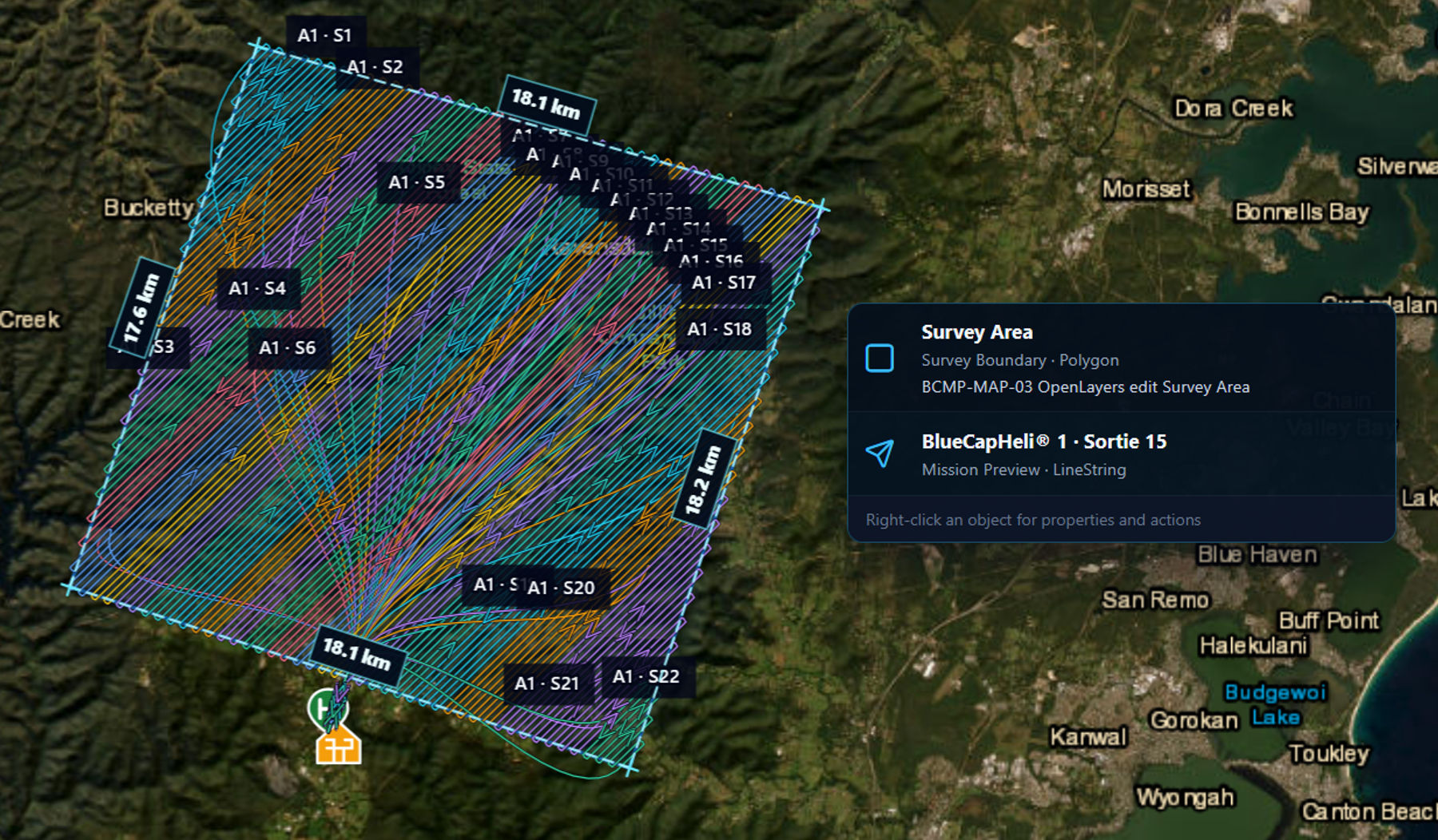
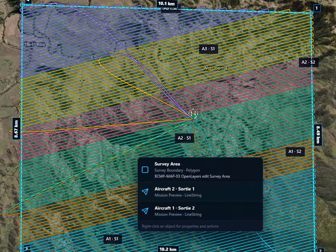
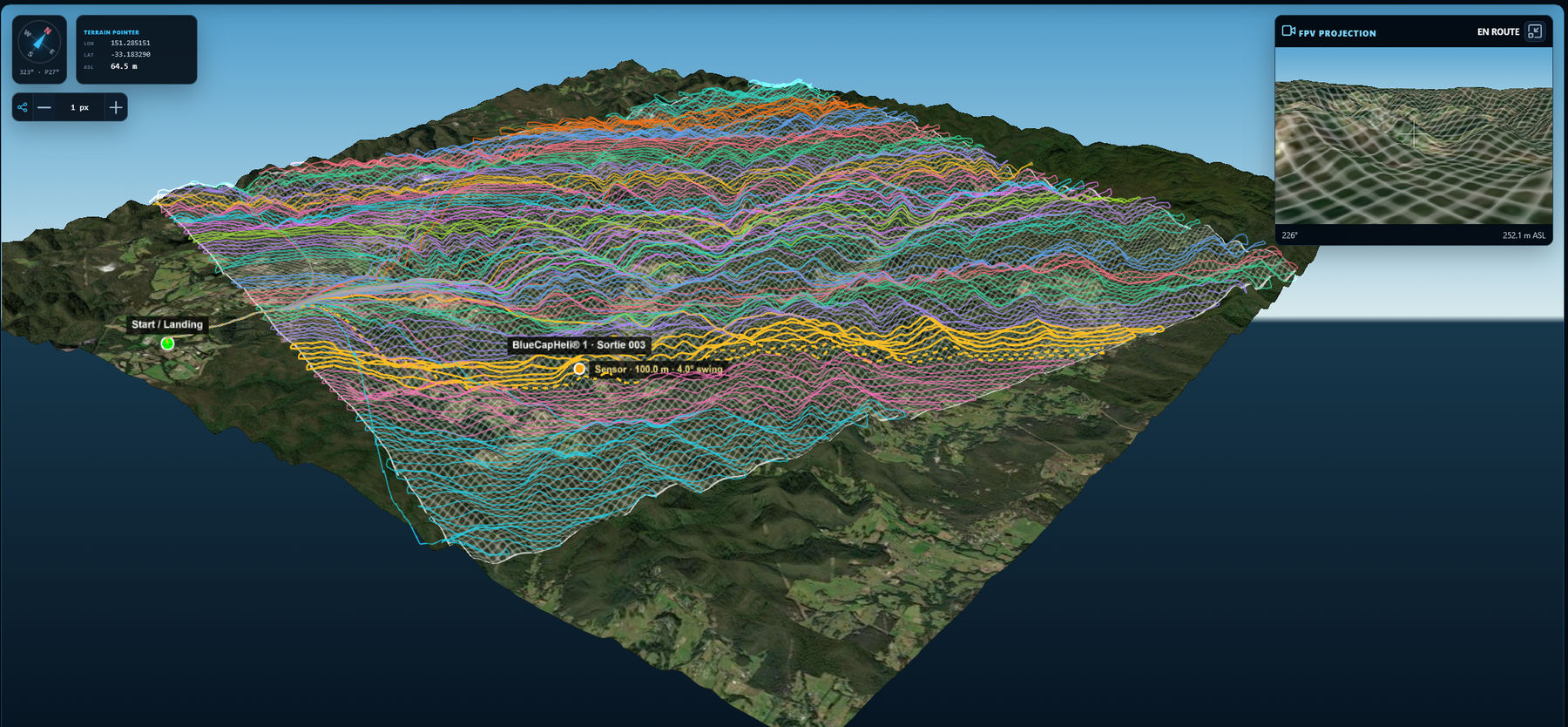
The 2D view documents coverage and sortie allocation at a 200 pts/m² planning target. The 3D view checks the same 18 × 18 km class of mission against terrain at 100 m sensor AGL and 180 m line spacing. These Portal views are planning evidence, not a substitute for the density, speed, overlap and deliverables confirmed in the quotation.
Select the area and useful point-density target above for a current reference Quote range including mobilisation.
Indicative like-for-like planning scenario for a current crewed-aircraft quotation. It is not presented as a fixed market tariff.
Compare the same density, accuracy, ground-return, classification and mobilisation scope before judging commercial differences.
A crewed aircraft can map thousands of square kilometres per day when collecting low-density regional elevation data. That is not equivalent to a detailed survey at approximately 180 points/m² nominal and centimetre-level acquisition accuracy. The useful comparison fixes the deliverable first, then compares daily coverage, mobilisation and project cost.
Three helicopters within one survey system acquire independently planned low-altitude blocks, combining regional production with terrain following and operation beneath higher cloud layers. Dual-orthogonal acquisition can tighten the stated accuracy further when the project requires it.
At comparable high density and accuracy, lower altitude, narrower swath, reduced speed or added overlap reduce the headline coverage available from low-density regional flying.
Density and absolute accuracy are separate measures, so both are stated. The BlueCap system row compares available daily throughput only. Require current quotations with the same density, accuracy, ground-return, classification and mobilisation scope before procurement.
Long-endurance sorties keep useful acquisition time high.
Less repositioning and fewer return-to-base cycles across the block.
The 330 km² reference block is planned across three productive field days at 100 km/h and 180 m lines.
Approximately 120 km²/day per helicopter on this historical comparison basis.
BlueCap owns acquisition, processing, QA and delivery as one system.
Set the project area and compare complete acquisition cycles for a long-endurance BlueCap system and a conventional multirotor payload.
BlueCapHeli® + BlueCapLidar®
3field days
18 h productive flight time
DJI Matrice + Zenmuse L2
52field days
308 h productive flight time
Both systems are compared on an eight-hour field day at 100 m AGL with turns, return-to-base and complete refuelling or battery-service cycles included. Field days round up, because a part-day still carries a full day of aircraft, crew and logistics cost. Actual productivity depends on terrain, canopy, weather, airspace and the required point density.
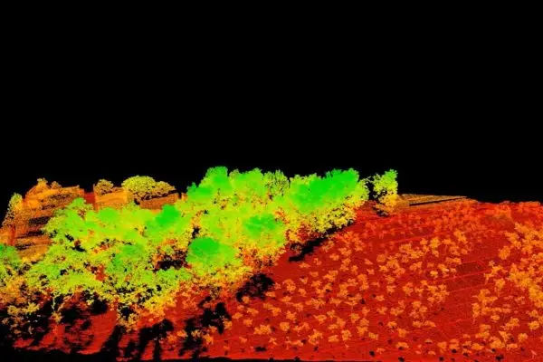
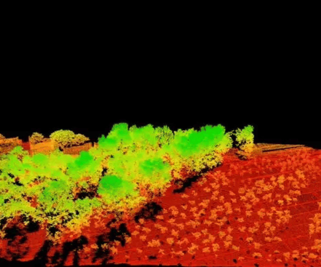
Choose the acquisition pattern from the terrain product required, not from scanner footprint alone. A second pass at 90° exchanges daily area for higher point density and a clearer understanding of the surface beneath tree canopy.
One set of parallel flight lines, typically spaced about 150 m apart with sidelap. This is the production-first pattern for broad areas and more open terrain.
Broad-area acquisition where field productivity is the priority. Particularly well suited to flat, lightly vegetated terrain such as deserts and open Western Australian bushland, where a single viewing axis meets the terrain-product requirement.
The complete block is flown twice: one full parallel grid, then a second full grid at 90°. Crossed coverage adds a second observation axis across every part of the site and four viewing directions rather than two.
Complementary pulse paths reduce direction-dependent occlusion behind tree crowns, scarps, rock faces, slopes and structures. They improve the opportunity for ground returns, make point geometry more uniform and support more stable classification and reconstruction of façades, outcrops and complex terrain.
Reference trade-off against single pass: field output is about half; density moves from ~230 to ~455 pts/m²; XY from 3–5 to 1.5–2.5 cm; Z from 4–8 to 2–4 cm; and canopy Z from ≤10–15 to ≤7 cm. These are project-design targets, not a universal probability of ground detection.The same measures stay aligned for direct comparison between both flight patterns.
The same survey blocks are compared on complete acquisition cycles. BlueCap uses 2.5-hour fuelled flight legs; Matrice uses battery flights with return-to-base service. Turns and complete refuelling or battery-service cycles are included. These are planning values, not guaranteed production rates.
carried by BlueCapHeli®
carried by DJI Matrice 300 RTK
carried by BlueCapHeli®
carried by DJI Matrice 300 RTK
carried by BlueCapHeli®
carried by DJI Matrice 300 RTK
| Survey block | System | Flight time | Field days | Flight cycles and field service |
|---|---|---|---|---|
| 10 × 10 km100 km² | BlueCapLidar®carried by BlueCapHeli® | 4h 30m | 1 | 2flight legs · 1 refuel |
| Zenmuse L2carried by DJI Matrice 300 RTK | 77h | 13 | 165battery cycles | |
| 20 × 20 km400 km² | BlueCapLidar®carried by BlueCapHeli® | 18h | 3 | 8flight legs · 7 refuels |
| Zenmuse L2carried by DJI Matrice 300 RTK | 307h 30m | 51 | 659battery cycles | |
| 30 × 30 km900 km² | BlueCapLidar®carried by BlueCapHeli® | 40h | 5 | 16flight legs · 15 refuels |
| Zenmuse L2carried by DJI Matrice 300 RTK | 692h | 115 | 1483battery cycles |
BlueCapLidar® first measures terrain, canopy and obstacles. That surface becomes a calculated magnetic drape used by BlueCapHeli®, BlueCapWinch® and the suspended QuSpin QTFM Gen 2 as one acquisition-control system.
BlueCapLidar® records a 285 × 160 m instantaneous window at 100 m AGL and builds the terrain and obstacle model.
Terrain, canopy and obstacles become a flyable sensor-height profile; 35 m sensor AGL is a common reference in difficult tropical and subtropical relief.
BlueCapWinch® actively manages the QuSpin QTFM Gen 2 while maintaining more than 20 m carrier-to-sensor separation.
Speed control and sensor-AGL QA follow the calculated surface to target a 1 m terrain-following corridor before interpretation.
BlueCap repeated one controlled vertical profile at four separate field locations. BlueCapHeli® ascended above a QuSpin QTFM Gen 2 suspended on a pre-measured 20 m line while the stripped tubular bird rotated freely at each 25–50 m sensor-AGL level. Every height refers to the sensor above ground, not carrier altitude.
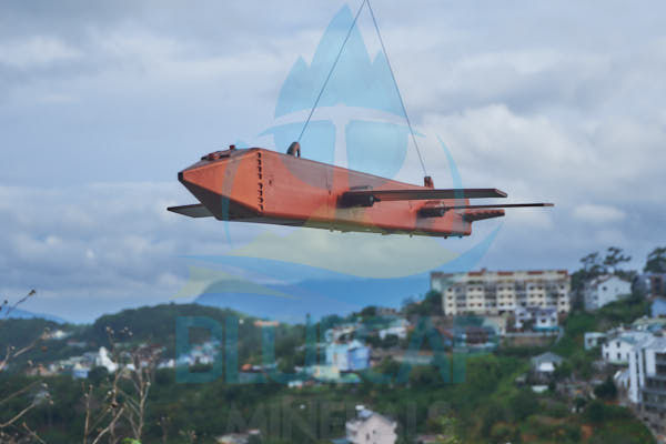
The response was repeated across separate sites rather than inferred from one location.
The carrier held horizontal position while only sensor-to-ground distance changed.
The helicopter increased height in one upward sequence; the 20 m suspension length remained fixed and sensor AGL was measured by range LiDAR.
The magnetic sensor never came closer than 20 m to the BlueCapHeli® airframe.
Interpretation boundary: the chart below normalises the 35 m response and applies the first-order relationship across the tested 25–50 m range. It interprets the controlled experiment; it is not the unpublished raw time series.
The curve sets the 35 m sensor-AGL response to 100% and applies the first-order 1/r³ relationship across the field-tested 25–50 m range. It interprets the controlled experiment; it is not a plot of the unpublished raw series from the four locations.
The engineers responsible for BlueCapLidar® also control its MCAP/MavROS 2 post-processing workflow. That connection keeps each LiDAR mapping requirement close to the payload, acquisition record and final terrain products.
In-house control avoids unnecessary third-party training, data adaptation and custom integration hours.

Flights record point clouds, telemetry and QA while the browser preview shows acquisition progress.
Flight strips are stitched with 20 m tile overlaps on a multi-node CPU cluster; about four hours is typical for one full flying day.
DTM, DSM, CHM, intensity and obstacle layers are generated, classified and quality controlled.
Agreed formats, metadata, coordinate reference system and vertical datum are checked for GIS, engineering or geophysical use.
Formats, coordinate reference system, vertical datum and tile structure are agreed for the client workflow before processing is finalised.
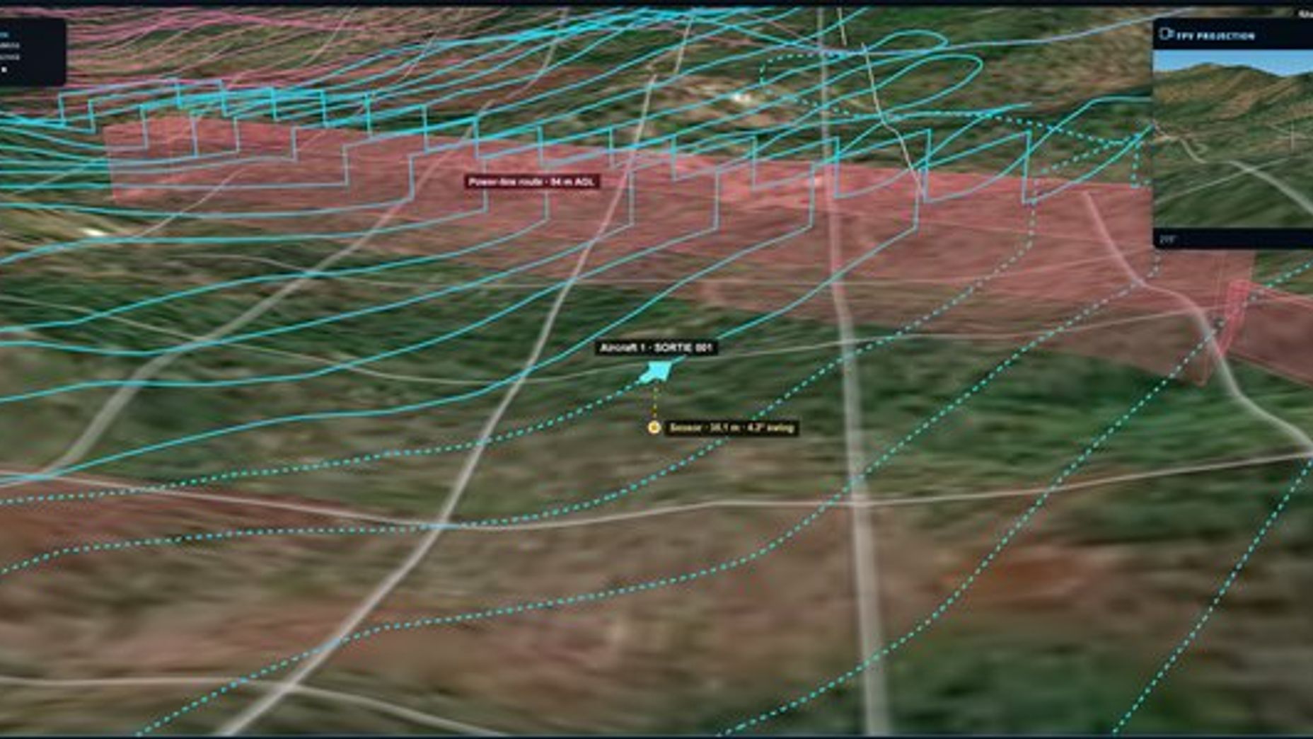
Technical review should start with measured data — the point cloud, terrain models, flight-path record and QA — rather than one headline scanner specification.
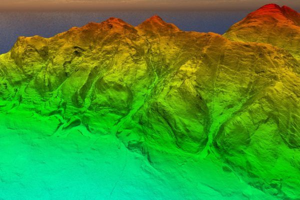
Each item answers a different technical question before a client commits to a larger programme.
Canopy penetration, ground returns and surface structure.
Pilot datasets · supplied on requestTerrain-model quality for drape planning and magnetic correction.
Prepared for the project area and datumDetection of powerlines, towers, buildings and tall vegetation.
Format matched to mission-planning workflowActual trajectory, instantaneous footprint and accumulated coverage geometry.
Used for internal planning and client reviewIndependent review by client geophysicists, GIS or engineering teams.
Selected projects · data agreement requiredRemote-project cost is driven by flyable hours, deployed crew days and repeat visits — not only the sensor day rate.
BlueCap is based on the Gold Coast, Queensland, so drone 3D mapping and LiDAR survey work in South East Queensland — the Gold Coast, Brisbane, Logan, Ipswich, the Scenic Rim and the Sunshine Coast — mobilises by road without freight or charter. The BlueCapHeli® system works as a long-endurance 3D survey drone: one mobilisation returns classified point clouds, bare-earth DTM and DSM terrain models, contours and other agreed 3D terrain products for mine and exploration sites, infrastructure and telecommunications corridors, flood, erosion and catchment terrain studies, forestry and rural land.
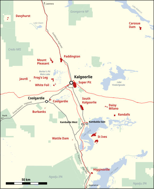
The same crew flies the rest of Queensland — the Bowen and Galilee basins, the North West Minerals Province around Mount Isa and Cloncurry, Central Queensland and Cape York — and every other Australian state and territory, from the Gold Coast base and equipment staged in Perth (Western Australia). Scope, approvals and deliverables are agreed per site: send the project boundary and the decision the terrain data has to support, and BlueCap will confirm coverage, point density and field time before mobilisation.
Project enquiry
Start with your survey area and the data you need. We’ll help define the scope, review terrain-aware 2D and 3D flight plans, and keep field progress, processed data and deliverables together in the BlueCap Survey Portal.
No software subscription fee for BlueCap service projects.